library(baseballr)
library(tidyverse)
library(brms)
library(bayestestR)
library(tidybayes)
library(scales)
library(gt)
library(hrbrthemes)
library(gtExtras)
library(ggrepel)
library(zoo)

# Set Stan options
options(mc.cores = parallel::detectCores())

season <- 2026

# ==============================================================================
# 1. SCRAPE & CONSTRUCT BOX SCORE DATASET
# ==============================================================================

mlb_batters <- fg_batter_leaders(
  startseason = season,
  endseason   = season,
  qual        = "n"
)

qual_det_batters <- mlb_batters %>%
  filter(team_name == "DET") %>%
  select(playerid, PlayerName, PA)

# Pull game logs for each batter
det_bat <- qual_det_batters %>%
  mutate(tmp_season = map(playerid, ~ fg_batter_game_logs(.x, season), .progress = TRUE))

# Unnest tmp_season cleanly without redundant coalescing
df_game_logs <- det_bat %>%
  select(tmp_season) %>%
  unnest(tmp_season) %>%
  janitor::clean_names() %>%
  mutate(
    batter_name = player_name,
    pa          = as.numeric(pa),
    ab          = as.numeric(ab),
    h           = as.numeric(h),
    doubles     = as.numeric(x2b),
    triples     = as.numeric(x3b),
    hr          = as.numeric(hr),
    bb          = as.numeric(bb),
    hbp         = as.numeric(replace_na(hbp, 0)),
    sf          = as.numeric(replace_na(sf, 0)),
    singles     = pmax(0, h - (doubles + triples + hr)),
    game_id     = paste(date, opp, sep = "_"),
    home_away   = if_else(str_detect(opp, "@"), "Away", "Home")
  ) %>%
  filter(pa > 0) %>%
  mutate(
    # Standard linear weights
    woba_numerator = (0.69 * bb) + (0.72 * hbp) + (0.88 * singles) +
      (1.25 * doubles) + (1.58 * triples) + (2.04 * hr),
    woba = woba_numerator / pa
  ) %>%
  select(game_id, batter = batter_name, pa, woba, home_away)

# ==============================================================================
# 2. BAYESIAN MODEL & ROPE EVALUATION FUNCTION
# ==============================================================================

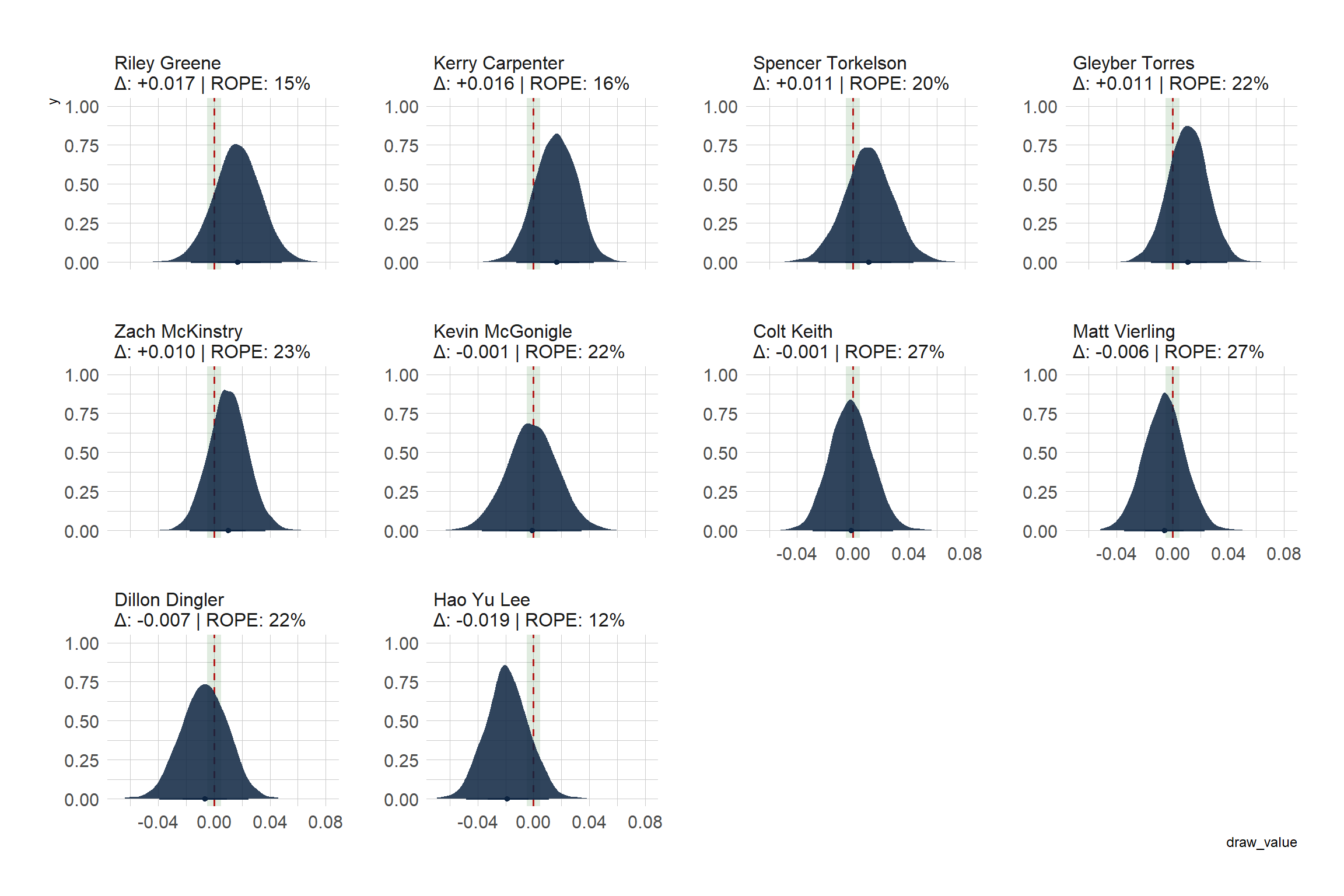
# Priors: Baseline wOBA ~ Normal(.315, .040); Delta ~ Normal(0, .020)
brms_priors <- c(
  prior(normal(0.315, 0.040), class = "Intercept"),
  prior(normal(0.000, 0.020), class = "b", coef = "target_active"),
  prior(exponential(20),      class = "sd"),
  prior(exponential(15),      class = "sigma")
)

ROPE_LOWER <- -0.005
ROPE_UPPER <-  0.005

fit_and_test_rope <- function(target_player, logs) {
  # Flag games the target started (>= 3 PA)
  target_starts <- logs %>%
    filter(batter == target_player) %>%
    group_by(game_id) %>%
    summarize(target_started = as.integer(any(pa >= 3)), .groups = "drop")

  all_games <- tibble(game_id = unique(logs$game_id))

  presence_map <- all_games %>%
    left_join(target_starts, by = "game_id") %>%
    mutate(target_active = replace_na(target_started, 0L))

  # Filter out target player's own PAs to isolate the rest of the lineup
  model_data <- logs %>%
    filter(batter != target_player) %>%
    left_join(presence_map, by = "game_id")

  presence_counts <- table(presence_map$target_active)
  if (length(presence_counts) < 2 || min(presence_counts) < 5) {
    message(paste("Skipping", target_player, "- insufficient games with/without."))
    return(NULL)
  }

  # Fit precision-weighted mixed model
  fit <- brm(
    woba | resp_weights(pa) ~ target_active + home_away +
      (1 + target_active | batter) +
      (1 | game_id),
    data    = model_data,
    family  = gaussian(),
    prior   = brms_priors,
    chains  = 4,
    iter    = 2000,
    warmup  = 1000,
    control = list(adapt_delta = 0.95),
    backend = "cmdstanr",
    refresh = 0,
    silent  = 2
  )

  draws <- as_draws_df(fit)
  b_target <- draws$b_target_active

  # Calculate 95% Highest Density Interval (HDI) using explicit namespace
  hdi_res <- bayestestR::hdi(b_target, ci = 0.95)

  # Compute percentage of posterior mass inside the ROPE
  rope_res <- bayestestR::rope(b_target, range = c(ROPE_LOWER, ROPE_UPPER), ci = 0.95)

  decision <- case_when(
    hdi_res$CI_low > ROPE_UPPER | hdi_res$CI_high < ROPE_LOWER ~ "Reject Null (Real Effect)",
    hdi_res$CI_low >= ROPE_LOWER & hdi_res$CI_high <= ROPE_UPPER ~ "Accept Null (Negligible)",
    TRUE ~ "Undecided (Noisy / Underpowered)"
  )

  # Return both summary row and raw posterior draws for plotting
  list(
    summary = tibble(
      player        = target_player,
      woba_without  = mean(draws$b_Intercept),
      woba_with     = mean(draws$b_Intercept + b_target),
      delta         = mean(b_target),
      hdi_lower     = hdi_res$CI_low,
      hdi_upper     = hdi_res$CI_high,
      rope_pct      = rope_res$ROPE_Percentage,
      decision      = decision
    ),
    draws = tibble(
      player = target_player,
      delta  = b_target
    )
  )
}

# ==============================================================================
# 3. RUN ACROSS REGULARS (>= 200 PA)
# ==============================================================================

qualifying_players <- df_game_logs %>%
  group_by(batter) %>%
  summarize(total_pa = sum(pa), .groups = "drop") %>%
  filter(total_pa >= 200) %>%
  pull(batter)

rope_results_raw <- qualifying_players %>%
  map(fit_and_test_rope, logs = df_game_logs, .progress = TRUE) %>%
  compact()

# Separate into summary table and draw tibbles
rope_results <- map_dfr(rope_results_raw, ~ .x$summary) %>%
  arrange(desc(delta))

all_draws <- map_dfr(rope_results_raw, ~ .x$draws)

# ==============================================================================
# 4. GT TABLE
# ==============================================================================

spillover_table <- rope_results %>%
  mutate(
    hdi_formatted = sprintf("[%+.3f, %+.3f]", hdi_lower, hdi_upper)
  ) %>%
  select(
    player,
    woba_without,
    woba_with,
    delta,
    hdi_formatted,
    rope_pct,
    decision
  ) %>%
  gt() %>%
  tab_header(
    title    = md("**Detroit Tigers: Lineup Spillover Effects (ROPE Hypothesis Test)**"),
    subtitle = "Bayesian test of practical equivalence: ROPE = [-0.005, +0.005] wOBA"
  ) %>%
  cols_label(
    player        = "Player",
    woba_without  = "Rest wOBA (Without)",
    woba_with     = "Rest wOBA (With)",
    delta         = "Mean Δ wOBA",
    hdi_formatted = "95% HDI",
    rope_pct      = "% in ROPE",
    decision      = "Hypothesis Test Verdict"
  ) %>%
  fmt_number(
    columns  = c(woba_without, woba_with),
    decimals = 3
  ) %>%
  fmt_number(
    columns    = delta,
    decimals   = 3,
    force_sign = TRUE
  ) %>%
  fmt_percent(
    columns  = rope_pct,
    decimals = 1
  ) %>%
  data_color(
    columns   = delta,
    direction = "column",
    palette   = c("#B31B1B", "#FDFDFD", "#1B5E20"),
    domain    = c(-0.035, 0.035)
  ) %>%
  text_transform(
    locations = cells_body(columns = decision),
    fn = function(x) {
      map_chr(x, function(val) {
        if (str_detect(val, "Reject Null")) {
          "<span style='color: #1B5E20; font-weight: bold;'>Reject Null (Real Effect)</span>"
        } else if (str_detect(val, "Accept Null")) {
          "<span style='color: #0D47A1; font-weight: bold;'>Accept Null (Equivalent to 0)</span>"
        } else {
          "<span style='color: #757575;'>Undecided (Underpowered)</span>"
        }
      })
    }
  ) %>%
  cols_align(
    align   = "center",
    columns = c(woba_without, woba_with, delta, hdi_formatted, rope_pct, decision)
  ) %>%
  cols_align(
    align   = "left",
    columns = player
  ) %>%
  tab_source_note(
    source_note = md(
      "*Decision Rule: 95% HDI outside ROPE rejects the null; 95% HDI entirely within ROPE accepts the null; overlap is undecided. Prior: Delta ~ N(0, 0.020).*"
    )
  ) %>%
  opt_row_striping() %>%
  tab_options(
    heading.title.font.size    = px(18),
    heading.subtitle.font.size = px(13),
    column_labels.font.weight  = "bold",
    table.font.size            = px(13)
  )

# Render table
spillover_table